Tutorial 2: Image Plane Positions

:::info Migrated from Old Wiki This tutorial has been enhanced with content from the old GLEE wiki. Content should be double-checked for accuracy. :::

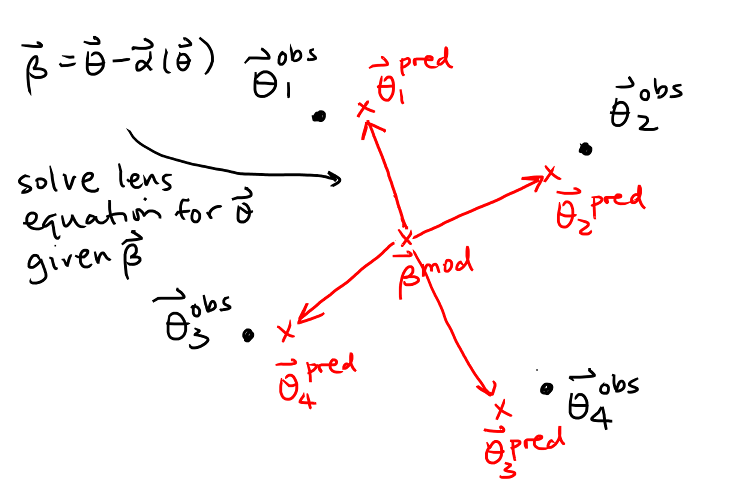
In Tutorial 1, we created a model that fits well to the source plane positions. While this provides a strong starting model, it can introduce issues like the over- or under-prediction of images.

Our next step is to optimise the model in the image plane. This produces a more realistic, robust model that accurately predicts the correct number of images.

$$\chi^2_{\text{im}} = \sum_{i=1}^{N_{\text{im}}} \frac{\left| \vec{\theta}_i^{\text{obs}} - \vec{\theta}_i^{\text{mod}} \left( \vec{\eta}, \vec{\beta}^{\text{mod}} \right) \right|^2}{\sigma_i^2}$$

Where:

• $\vec{\theta}_i^{\text{obs}}$ is the observed position of the $i$-th quasar image (obtained by fitting a PSF light profile to the observed images).
• $\vec{\theta}_i^{\text{mod}}$ is the predicted position of the $i$-th quasar image.
• $N_{\text{im}}$ is the image multiplicity (e.g., 4 for a quad).
• $\vec{\eta}$ are the mass model parameters.
• $\sigma_i$ is the positional uncertainty.

Why Image Plane?

Source-plane modelling is computationally cheap but has a subtle bias: it can produce models that predict the wrong number of images (e.g., 5 images for a quad system) because it does not check whether the model actually reproduces the observed image multiplicity. Image-plane modelling avoids this by comparing model-predicted image positions directly to observations, enforcing the correct image geometry.

Step 1: Update the Config File

To switch to image plane modelling, update the chi2type in the global parameters of your config file:

chi2type 2

Everything else in the config (lens parameters, source positions, step sizes) can remain the same as the best-fit result from Tutorial 1.

:::tip Starting point Use the best-fit config file from Tutorial 1 (output of the last siman run) as your starting point for Tutorial 2. This ensures you begin close to a good model and avoid long initial optimisation. :::

Step 2: Siman/MCMC Cycle

Repeat the same optimisation cycle as in Tutorial 1:

1. Run simulated annealing to find the best-fit parameters:

   glee.py minimise -o configfile_img2 configfile_img

2. Check img_chi2 (image-plane chi-squared):

   glee.py chi2 -c img -- configfile_img2

3. Run MCMC to sample the posterior:

   glee.py -v 1 mcmc configfile_img2

4. Save the best-fit iteration as a new config and update the covariance matrix.

5. Repeat until img_chi2 is thoroughly stable and minimised.

:::note Convergence A well-converged image-plane model should have img_chi2 / dof close to 1 and stable MCMC chains with an acceptance rate near 25%. :::

Step 3: Verify the Solution

Use glee.py analyse to compare predicted and observed image positions:

glee.py analyse configfile_img2

This prints the predicted image positions alongside the observed ones, letting you check residuals directly. Once the model is converged, proceed to Tutorial 3 to add surface brightness fitting.

---

Advanced: Parameter Linking

As your models become more complex (e.g., multiple lens components, light + mass), you may want to link parameters between different components to enforce physical constraints or reduce model degeneracy.

Syntax

Use label: to name a parameter, then link: to tie another parameter to it:

lenses_vary 2
    piemd
    4.000000  #x-coord   flat:3.8,4.2   step:0.05  label:lens_x
    4.000000  #y-coord   flat:3.8,4.2   step:0.05  label:lens_y
    # ... other parameters
    
    shear
    0.050000  #magnitude  flat:0,0.3     step:0.01
    1.200000  #theta      link:mass_pa   a:0,1,1

The a:a1,a2,a3 Coefficients

The link: syntax follows the transformation:

$$y_{\text{linked}} = a_1 + a_2 \cdot x_{\text{labeled}}^{a_3}$$

Common Use Cases:

Use Case	a: values	Formula	Example
Identity (same value)	a:0,1,1	$y = x$	Shear PA = lens PA
Offset	a:0.5,1,1	$y = x + 0.5$	Secondary lens offset from primary
Scale	a:0,0.5,1	$y = 0.5x$	Core radius proportional to Einstein radius
Opposite sign	a:0,-1,1	$y = -x$	Mirror across axis
Quadratic	a:0,1,2	$y = x^2$	Non-linear relationships

Example: Mass-Follows-Light

Force a mass profile center to track a light profile center:

lights_vary 1
    sersic
    4.000000  #x-coord   flat:3.8,4.2   step:0.05  label:gal_x
    4.000000  #y-coord   flat:3.8,4.2   step:0.05  label:gal_y
    # ... other Sérsic parameters

lenses_vary 1
    piemd
    4.000000  #x-coord   link:gal_x     a:0,1,1
    4.000000  #y-coord   link:gal_y     a:0,1,1
    # ... other PIEMD parameters

Now the PIEMD mass centroid will always match the Sérsic light centroid, reducing free parameters from N+2 to N.

Example: Align Shear with Lens PA

Constrain external shear to be aligned with the lens major axis:

lenses_vary 2
    spemd
    4.000000  #x-coord   flat:3.8,4.2   step:0.05
    4.000000  #y-coord   flat:3.8,4.2   step:0.05
    0.700000  #b/a       flat:0.5,1.0   step:0.05
    1.500000  #theta     flat:0,6.28    step:0.1   label:mass_pa
    0.800000  #theta_e   flat:0.5,3.0   scale:     step:0.05
    
    shear
    0.050000  #magnitude  flat:0,0.3     step:0.01
    1.500000  #theta      link:mass_pa   a:0,1,1

Now the shear orientation will track the SPEMD orientation.

Nested Linking

You can link parameters in chains: x → y → z

:::caution Order Matters! GLEE updates non-linked parameters first, then applies links in the order they appear in the config file.

Case I (recommended):

x    label:L1
y    link:L1    label:L2
z    link:L2

Result: z gets the updated value of y (which is updated from x)

Case II (problematic):

x    label:L1
z    link:L2
y    link:L1    label:L2

Result: z gets the old value of y (before it was updated from x)

Best practice: Declare links in dependency order (base parameters first, derived parameters last). :::

When to Use Linking

• Reducing degeneracies: When mass and light are expected to trace each other
• Enforcing symmetry: When components should share a PA or axis ratio
• Multiplane lensing: Link higher-redshift lens positions to their source positions (see Tutorial 5)
• Physical priors: When two parameters are expected to correlate (e.g., core radius ~ Einstein radius)

:::tip Performance Boost Linking reduces the effective number of free parameters, speeding up MCMC convergence and reducing parameter space volume. :::