Tutorial 1: Source Plane Positions

:::info Migrated from Old Wiki This tutorial has been enhanced with content from the old GLEE wiki. Content should be double-checked for accuracy. :::

:::tip Prerequisite Before you start, make sure you have familiarised yourself with the structure of the GLEE Configfile and glee.py. :::

Introduction

Gravitational lens modelling often requires fitting lens parameters by comparing observed image positions with those predicted by a lens model. One approach is working in the source plane, where each observed image position is mapped back to a position in the source plane using a trial lens model. A good model should map all observed images back to the exact same source location.

When modelling with source plane positions, we search for lens model parameters $\vec{\eta}$ and a modelled source position $\vec{\beta}^{\text{mod}}$ that minimise the following $\chi^2$:

$$\chi^2_{\text{sr}} = \sum_{i=1}^{N_{\text{im}}} \frac{\left| \vec{\beta}_i(\vec{\theta}_i^{\text{obs}}; \vec{\eta}) - \vec{\beta}^{\text{mod}}(\vec{\theta}_i^{\text{obs}}; \vec{\eta}) \right|^2}{\left( \frac{\sigma_i}{\sqrt{\mu_i}} \right)^2}$$

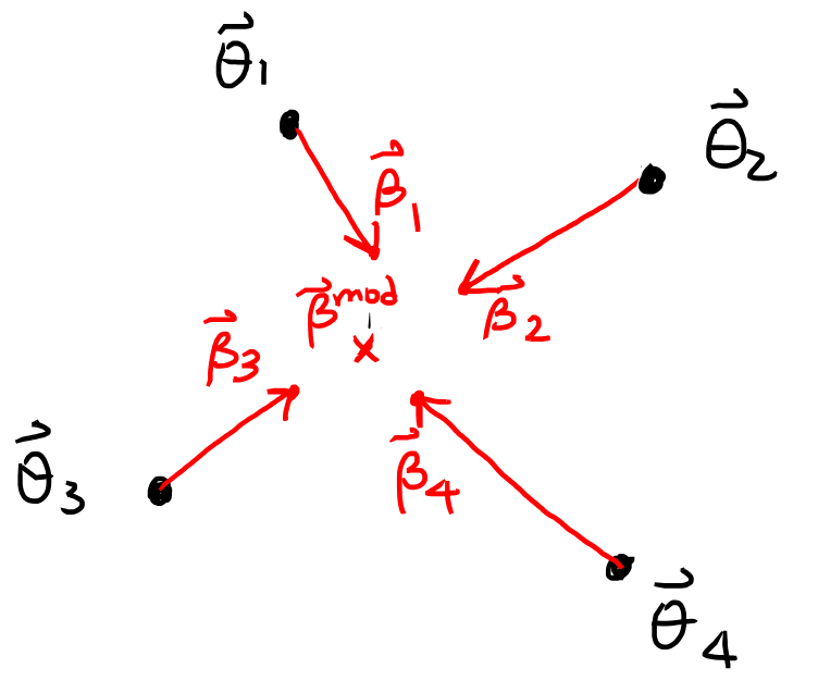
Where:

• $\vec{\beta}_i$: the inferred source position from the $i$-th image,
• $\vec{\beta}^{\text{mod}}$: the modelled source position (often the weighted mean),
• $\mu_i$: magnification of image $i$,
• $\sigma_i$: positional uncertainty of image $i$ on the image plane,
• $N_{\text{im}}$: number of observed lensed images.

This method is computationally efficient and useful for initial parameter exploration, though it comes with caveats (e.g., over/under-predicting images).

1. Global Parameters

At the top of your config file, define the global settings, establishing chi2type 1 to enable source-plane optimisation.

chi2type        1
minimiser       siman
seed            1

siman_iter      1
siman_nT        1000
siman_dS        10
siman_Sf        1.1
siman_k         2
siman_Ti        10
siman_Tf        1.1
siman_Tmin      1

mcmc_n          100000
mcmc_dS         0.5
mcmc_dSini      0
mcmc_k          2

Rsoft           1e-05

2. Lens Mass Parameters

Under lenses_vary 2, define a two-component lens model consisting of an elliptical power law (epl) and an external shear component.

lenses_vary 2
    epl
    4.000000  #x-coord   flat:3.8,4.2   step:0.1
    4.000000  #y-coord   flat:3.8,4.2   step:0.1
    0.700000  #b/a       flat:0.1,1     step:0.1
    1.500000  #theta     flat:0,6.3     step:0.1
    0.800000  #theta_e   flat:0.5,3  scale:  step:0.1
    1.500000  #gam       flat:0.3,0.7  step:0.1

    shear
    0.070000  #magnitude  flat:0,0.6  step:0.1
    0.800000  #theta      flat:0,6.3  step:0.1

3. Source and Image Positions

Convert the observed quasar image positions from pixel coordinates to arcseconds:

sources 1
    Dds/Ds    1.000000  exact:
    source weighted
    srcx      3.700000  exact:
    srcy      3.700000  exact:
    4
    4.3200000   3.9200000  error:0.04
    5.6000000   4.7200000  error:0.04
    5.1200000   5.6000000  error:0.04
    4.2400000   5.3600000  error:0.04

3a. Source Position Options

GLEE offers four methods to determine the source position from the observed image positions. Specify the option under Dds/Ds:

sources 1
    Dds/Ds    1.000000  exact:
    source OPTION         # ← Choose one: mean | weighted | best | parameter
    srcx      3.700000  exact:
    srcy      3.700000  exact:

Option	Description	When to Use
mean	Unweighted mean of mapped image positions	Quick initial exploration; all images have similar magnification
weighted	Mean weighted by magnification $\mu_i$	Recommended default — downweights highly magnified (distorted) images
best	Source position that minimizes $\chi^2_{\text{sr}}$	When source position itself is a constraint (e.g., from independent data)
parameter	Treat srcx, srcy as free parameters	Advanced: when source position has priors or is linked to another source

:::note Automatic Updates For mean, weighted, or best, GLEE automatically updates srcx and srcy in the output config file to the computed optimal values. :::

3b. Positional Uncertainties

Specify observational uncertainties using the error: keyword. GLEE supports both circular and elliptical error regions.

Circular Errors (Isotropic)

For symmetric positional uncertainty:

4.3200000   3.9200000  error:0.04

This represents a 2D Gaussian error circle with $\sigma = 0.04$ arcsec in both x and y directions.

Elliptical Errors (Anisotropic)

For elongated uncertainties (common along arcs):

error:r_major,r_minor,theta

• r_major: semi-major axis (arcsec)
• r_minor: semi-minor axis (arcsec)
• theta: position angle in radians (CCW from +x axis)

Example: Error ellipse with major axis = 0.10", minor axis = 0.03", oriented 45° from +x:

5.1200000   5.6000000  error:0.10,0.03,0.785

Mathematical Implementation

GLEE computes the image-plane positional $\chi^2$ for each image using the error matrix formalism. Given an error ellipse error:a,b,theta where $a = r_{\text{major}}$, $b = r_{\text{minor}}$:

1. Define error matrix $\mathbf{E}$ (in principal axes):

   $$\mathbf{E} = \begin{pmatrix} a^2 & 0 \\ 0 & b^2 \end{pmatrix}$$

2. Define rotation matrix $\mathbf{R}$:

   $$\mathbf{R} = \begin{pmatrix} -\cos\theta & -\sin\theta \\ \sin\theta & -\cos\theta \end{pmatrix}$$

3. Transform to observed frame:

   $$\mathbf{T} = \mathbf{R}^{-1} \mathbf{E} \mathbf{R}$$

4. Invert to get covariance matrix:

   $$\mathbf{S} = \mathbf{T}^{-1} = \begin{pmatrix} S_{11} & S_{12} \\ S_{21} & S_{22} \end{pmatrix}$$

5. Compute chi-squared for image $i$ with observed position $(x, y)$ and predicted position $(x_P, y_P)$:

   $$\begin{align} \Delta x &= x - x_P \\ \Delta y &= y - y_P \\ \chi^2_i &= \Delta x^2 \cdot S_{11} + 2\Delta x \Delta y \cdot \frac{S_{12} + S_{21}}{2} + \Delta y^2 \cdot S_{22} \end{align}$$

:::tip Special Case: $\theta = 0$ When the error ellipse is aligned with the x-axis ($\theta = 0$):

$$\chi^2_i = \frac{\Delta x^2}{a^2} + \frac{\Delta y^2}{b^2}$$

:::

3c. Flux Constraints (Optional)

If flux measurements are available, constrain the model using magnification $\chi^2$ (chi2type 4).

Basic Flux Syntax

sources 1
    Dds/Ds    1.000000  exact:
    source weighted
    4
    4.3200000   3.9200000  error:0.04  flux:10.0,2.0
    5.6000000   4.7200000  error:0.04  flux:5.0,1.5
    5.1200000   5.6000000  error:0.04  flux:8.2,1.8
    4.2400000   5.3600000  error:0.04  flux:3.1,0.9

• First value: Observed flux (arbitrary units)
• Second value: Flux uncertainty

Magnification Chi-Squared Formula

$$\chi^2_{\text{mag}} = \sum_{i,j} \left( \frac{f_{i,j} - \mu_{i,j}^{\text{model}} \cdot s_i^{\text{model}}}{\sigma_{i,j}} \right)^2$$

where:

• $f_{i,j}$: observed flux of image $j$ in system $i$
• $\mu_{i,j}^{\text{model}}$: model magnification
• $s_i^{\text{model}}$: intrinsic source flux (computed as weighted mean)
• $\sigma_{i,j}$: flux uncertainty

Special Keywords for Flux Modeling

Central images (cusps/folds) can have extreme demagnification ($\mu \sim 0.01$), making source flux estimation numerically unstable. Use the central: flag to exclude them from the intrinsic flux calculation:

4.2400000   5.3600000  error:0.04  flux:0.5,0.2  central:

Non-detections can be modeled as upper limits using fluxlimit::

5.1200000   5.6000000  error:0.04  flux:0.1,0.05  fluxlimit:

This treats the flux value as an upper bound (the uncertainty is ignored).

:::warning Caution with Central Images Avoid using fluxlimit: on central images when the central mass density could be very high (e.g., supermassive black hole). GLEE may not find the central image, artificially inflating $\chi^2_{\text{img}}$ and wrongly rejecting plausible models. :::

4. Minimisation

Save the above sections in a config file and run a basic simulated annealing (siman):

glee.py minimise -o configfile2 configfile

To compare $\chi^2$ values before and after:

glee.py chi2 -c src -- configfile       # initial fit
glee.py chi2 -c src -- configfile2      # optimised fit

5. MCMC Optimisation

To sample the parameter space thoroughly, run MCMC on your new file:

glee.py -v 1 mcmc configfile2

This saves accepted iterations as a .mcmc file. Ensure mcmc_dS yields an acceptance ratio of ~0.25.

MCMC / Siman Cycle

Iteratively refine the model:

1. Run siman on the config file.
2. Run MCMC on the siman result (e.g., 100k iterations).
3. Save the best-fit iteration as a new config file.
4. Update the config with the new covariance matrix.
5. Recalculate $\chi^2$.

With this cycle, src_chi2 typically reduces to $\mathcal{O}(10^{-2})$. Use gleeview.py to verify that all images map back to a tiny central source region.

:::tip Next Step Once src_chi2 has converged, proceed to Tutorial 2: Image Plane Positions to refine your model using image-plane constraints. :::

---

6. Parameter Flags and Options

GLEE provides flexible parameter control through flags and keywords. Understanding these is essential for efficient optimization.

Common Parameter Flags

Flag	Syntax	Description	Use Case
flat:	flat:min,max	Flat (uniform) prior between bounds	Standard optimization with physical bounds
gauss:	gauss:mean,sigma	Gaussian prior	Incorporate external constraints (e.g., velocity dispersion)
noprior:	noprior:	No explicit prior (unbounded)	Exploratory runs; use with care
exact:	exact:	Fixed parameter (not varied)	Hold values constant (e.g., known redshifts)
log:	log:	Sample in log-space	Parameters spanning orders of magnitude (e.g., core radius)
step:	step:0.1	MCMC step size	Tune acceptance rate (~0.25 optimal)
scale:	scale:	Profile-specific normalization	Convert strength → Einstein radius (profile-dependent)
label:	label:name	Assign identifier for linking	Enable parameter relationships
link:	link:name a:a,b,c	Link to labeled parameter	Enforce $y = a + b \cdot x^c$ relationship

Example: Tuning an EPL Profile

lenses_vary 1
    epl
    4.000000  #x-coord   flat:3.8,4.2   step:0.05  label:lens_x
    4.000000  #y-coord   flat:3.8,4.2   step:0.05  label:lens_y
    0.700000  #b/a       flat:0.5,1.0   step:0.05
    1.500000  #theta     flat:0,6.28    step:0.1
    0.800000  #theta_e   flat:0.5,3.0   scale:  step:0.05
    1.500000  #gam       flat:1.8,2.2   step:0.02  gauss:2.0,0.1

Interpretation:

• x, y coords: Flat prior with tight bounds; labeled for linking to other components
• theta_e: Uses scale: to interpret value as Einstein radius (not raw normalization)
• gam (slope): Gaussian prior centered at 2.0 (isothermal) with $\sigma = 0.1$

The scale: Keyword

The scale: keyword modifies how profile strength parameters are interpreted:

Without scale:: The parameter is the raw normalization of the convergence.

With scale:: The parameter is the effective Einstein radius $\theta_E$.

For PIEMD:

• Without scale:: $E_0 = \theta_E$ directly
• With scale:: $E_0 = \frac{\theta_E^2}{\sqrt{\theta_E^2 + w^2} - w}$

:::tip When to Use scale: Use scale: when you want the parameter to represent a directly measurable quantity (Einstein radius from observed image separation) rather than an abstract normalization. :::

Parameter Linking

Link parameters between different components using label: and link::

lenses_vary 2
    piemd
    4.000000  #x-coord   flat:3.8,4.2   step:0.05  label:mass_x
    4.000000  #y-coord   flat:3.8,4.2   step:0.05  label:mass_y
    # ... other parameters

    shear
    0.050000  #magnitude  flat:0,0.3     step:0.01
    1.200000  #theta      link:mass_pa   a:0,1,1   # same PA as PIEMD

The link: syntax: link:label_name a:offset,multiply,exponent

$$y_{\text{linked}} = \text{offset} + \text{multiply} \times x_{\text{labeled}}^{\text{exponent}}$$

Example: link:lens_x a:0.1,1,1 → Offset by +0.1 arcsec from labeled lens_x

---

7. Convergence Diagnostics

Assessing Source-Plane Fit Quality

After MCMC, check if the model has converged:

glee.py chi2 -c src -- configfile_mcmc_best

Good convergence indicators:

• $\chi^2_{\text{src}} / \text{dof} \lesssim 0.1$
• $\chi^2_{\text{img}} / \text{dof} \lesssim 1$ (for sanity check)
• All images map to a compact source region (verify with gleeview.py)

Poor convergence indicators:

• $\chi^2_{\text{src}} / \text{dof} > 1$ → Model cannot map images to common source
• MCMC acceptance rate $\ll 0.25$ → Step sizes too large (reduce mcmc_dS)
• MCMC acceptance rate $\gg 0.25$ → Step sizes too small (increase mcmc_dS)

Covariance Matrix Analysis

After MCMC, generate a covariance matrix to assess parameter degeneracies:

glee.py covar -H 10000 configfile.mcmc

• -H 10000: Burn-in (discard first 10,000 accepted samples)
• Outputs: configfile.cov (covariance matrix file)

Using the covariance:

mcmc_n          100000
mcmc_dS         0.5
mcmc_dSini      0
mcmc_k          2
sampling_cov    configfile.cov   # ← Use covariance for efficient sampling

This enables adaptive MCMC using the covariance structure, improving mixing and convergence.

When to Move to Image Plane

Source-plane modeling has known limitations:

• Can over/under-predict the number of images
• Positional uncertainties propagate through magnification factor
• Not robust for complex mass distributions

Transition to Tutorial 2 when:

1. $\chi^2_{\text{src}}$ has plateaued (no longer improving)
2. You've iterated siman → MCMC → covar → MCMC at least 2-3 times
3. You're ready for a more physically robust constraint (image-plane positions)

:::tip Best Practice Use source-plane modeling to get initial parameter estimates and a rough covariance matrix, then switch to image-plane fitting for the final model. :::