Tutorial 0: Preliminary Data

:::info Migrated from Old Wiki This tutorial has been enhanced with content from the old GLEE wiki. Content should be double-checked for accuracy. :::

:::note Prerequisites This tutorial assumes familiarity with handling .fits files, DS9, and Python. :::

In this tutorial, we will generate the data required to model a gravitational lens system.

System to be Modelled

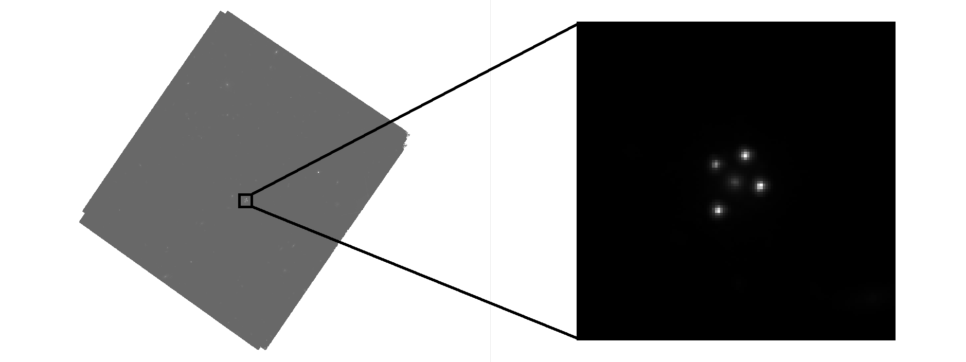
We will start by modelling a quad system—a system where one point source is lensed into four observable images. This specific system is known as WG0214-2105.

(Dataset download link to be added here).

We recommend generating these files manually using astropy or similar tools to get familiar with the file structures.

1. Lens Cutout

Observation data includes a lot of information which is not needed, so in order to model efficiently we require a restricted cutout of the system.

Python Example: Creating a Cutout

from astropy.io import fits
from astropy.nddata import Cutout2D
from astropy.wcs import WCS
import numpy as np

# Load the full science image
hdul = fits.open('full_science_image.fits')
data = hdul[0].data
wcs = WCS(hdul[0].header)

# Define cutout center (pixel coordinates) and size
center = (1024, 2048)  # (x, y) in pixels
size = (240, 240)       # Width, height in pixels

# Create cutout
cutout = Cutout2D(data, center, size, wcs=wcs)

# Save cutout to new FITS file
fits.writeto('sci.fits', cutout.data, cutout.wcs.to_header(), overwrite=True)
print(f"Cutout saved: shape = {cutout.data.shape}")

:::tip Choosing Cutout Size

• Include the full lens system + arc with ~20-30 pixel buffer
• Avoid nearby contaminating sources when possible
• Typical cutout: 100-300 pixels per side :::

2. Arc Mask

This FITS file contains a mask covering the extended arc from the lensed source. Pixels with a value of 1 are masked and part of the arc, while those with a value of 0 are unmasked. Aim to cover the full extent of the source galaxy's light (the arc), but avoid making the mask too thick. Each pixel in the arc mask is inverted and regularized during the source reconstruction process, which is computationally expensive.

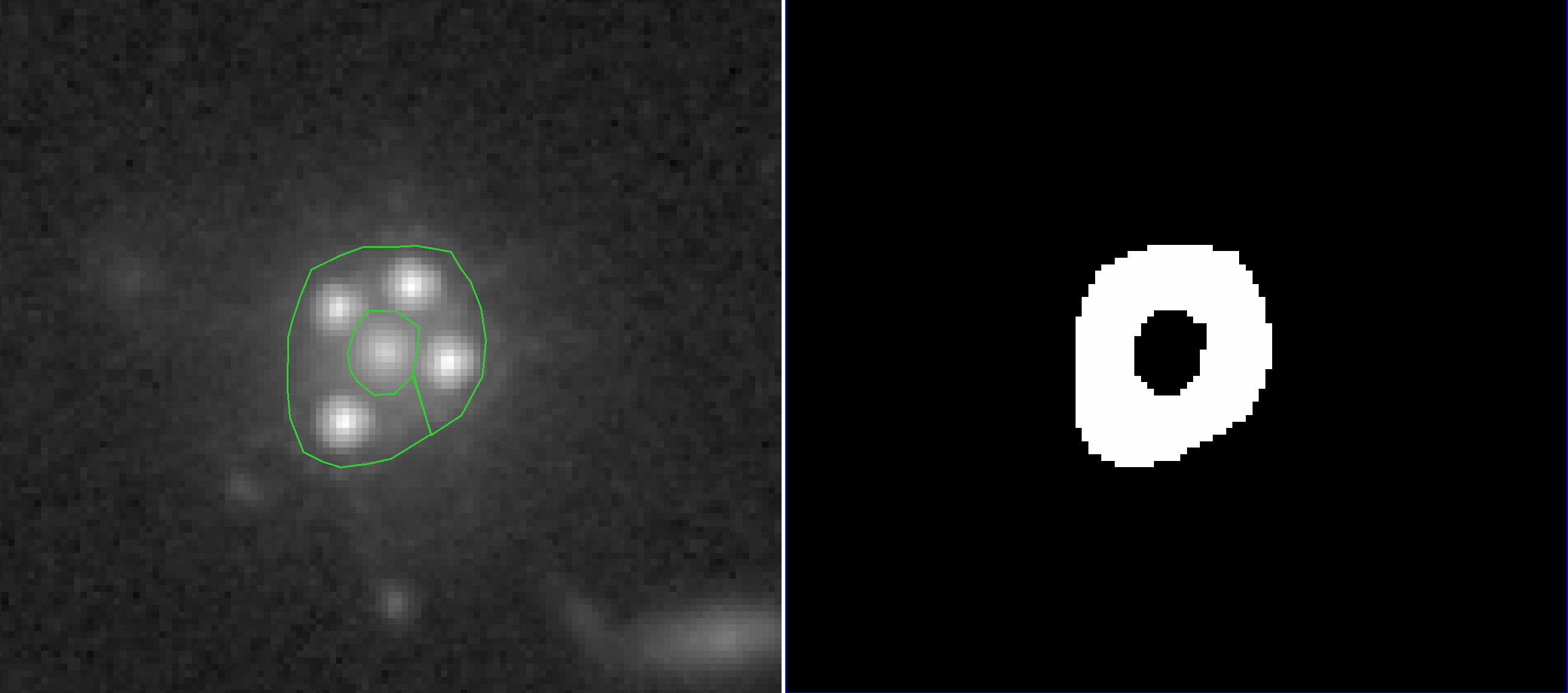Same cutout as above, but with a logarithmic scale. The arc region is marked in green, with the generated arc mask to the right.

Creating Arcmasks from DS9 Regions

GLEE provides a helper script to convert DS9 polygon regions to FITS masks:

getMaskInFitsFromDS9reg.csh arcmask.reg 240 240 arcmask.fits

Steps:

1. Open your science cutout in DS9
2. Use Region → Shape → Polygon to draw around the arc
3. Save region: Region → Save Regions (select Image coordinates, Physical system)
4. Ensure the region file has 4 header lines before the polygon coordinates (add #dummyline at the top if needed)
5. Run the script above (replace 240 240 with your cutout dimensions)

For multiple arcs, combine regions:

getMaskInFitsFromDS9reg.csh arc1.reg arc2.reg 240 240 arcmask_combined.fits

Python Alternative: Manual Mask Creation

from astropy.io import fits
import numpy as np
from matplotlib.path import Path

# Load science image to get shape
sci = fits.getdata('sci.fits')
ny, nx = sci.shape

# Define polygon vertices (pixel coordinates, 0-indexed)
# Example: arc vertices traced manually
vertices = np.array([
    [120, 80], [140, 75], [160, 78], [175, 85],
    [180, 95], [178, 110], [170, 120], [150, 125],
    [130, 122], [115, 110], [110, 95], [115, 85]
])

# Create grid of all pixel coordinates
y, x = np.mgrid[:ny, :nx]
points = np.vstack((x.flatten(), y.flatten())).T

# Create mask using matplotlib Path
path = Path(vertices)
mask = path.contains_points(points).reshape((ny, nx))

# Convert boolean to integer (1 inside polygon, 0 outside)
arcmask = mask.astype(np.int16)

# Save to FITS
fits.writeto('arcmask.fits', arcmask, overwrite=True)
print(f"Arcmask created: {np.sum(arcmask)} pixels masked")

3. Lens Mask

This FITS file contains a mask that marks pixels to be included during the modelling process. Pixels with a value of 1 are masked and included, while those with a value of 0 are not. Essentially, any light that does NOT belong to the system is marked by 0.

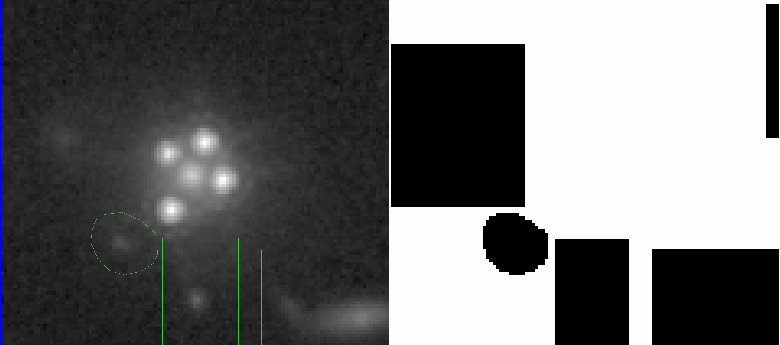Regions with light belonging to outside objects are boxed in green, with the generated lens mask to the right.

Python Example: Creating a Lens Mask

from astropy.io import fits
import numpy as np
from photutils.segmentation import detect_sources

# Load science cutout
sci = fits.getdata('sci.fits')

# Start with all pixels included
lensmask = np.ones_like(sci, dtype=np.int16)

# Option 1: Manually exclude contaminating sources (rectangular regions)
# Example: exclude a bright star at pixel (50, 200)
lensmask[190:210, 40:60] = 0  # [y_min:y_max, x_min:x_max]

# Option 2: Use segmentation to auto-detect and exclude faint sources
from photutils.segmentation import detect_threshold
threshold = detect_threshold(sci, nsigma=2.0)
segm = detect_sources(sci, threshold, npixels=10)

# Identify the lens system segment ID (largest flux segment usually)
lens_id = np.argmax([np.sum(sci[segm.data == i]) for i in range(1, segm.nlabels+1)]) + 1

# Keep only the lens system segment + some buffer
lensmask_auto = (segm.data == lens_id).astype(np.int16)

# Dilate the mask slightly to include faint wings
from scipy.ndimage import binary_dilation
lensmask_dilated = binary_dilation(lensmask_auto, iterations=5).astype(np.int16)

# Save
fits.writeto('lensmask.fits', lensmask_dilated, overwrite=True)
print(f"Lensmask created: {np.sum(lensmask_dilated)} pixels included")

4. Error Map

To quantify the per-pixel uncertainty in the data, both background and photon noise contributions must be taken into account.

1. Background uncertainty is estimated by calculating the standard deviation of the image background (where no sources are present).
2. Poisson noise is computed using:

$$\sigma^2_{\text{Poisson, } (x,y)} = \left| \frac{I_{(x,y)}}{t_{(x,y)} \cdot G} \right|$$

where $I_{(x,y)}$ is the pixel intensity in counts per second, $t_{(x,y)}$ is the local exposure time (from the exposure map), and $G$ is the instrument gain.

The total pixel-wise uncertainty, $\sigma_{(x,y)}^2$, is then calculated as:

$$\sigma_{(x,y)}^2 = \begin{cases} \sigma_{\text{Background}}^2 + \sigma^2_{\text{Poisson, } (x,y)} & \text{if } \sigma_{\text{Poisson, } (x,y)} \geq 2 \times \sigma_{\text{Background}} \\ \sigma_{\text{Background}}^2 & \text{otherwise} \end{cases}$$

During extended source reconstruction, the uncertainty is artificially increased near quasar centroids such that the normalised residuals in the region are all under $1\sigma$, a process we call boosting. This diminishes the influence of the bright quasar regions, allowing for a more accurate reconstruction of the surrounding arcs.

Python Example: Creating an Error Map

from astropy.io import fits
import numpy as np
from astropy.stats import sigma_clipped_stats

# Load science image (counts/sec) and exposure map (seconds)
sci = fits.getdata('sci.fits')
exp_map = fits.getdata('exp_map.fits')

# Instrument parameters (example: HST/ACS WFC)
gain = 2.0  # electrons/ADU

# 1. Estimate background noise from empty region
# Use sigma-clipped statistics to avoid contamination from sources
mean, median, sigma_bkg = sigma_clipped_stats(sci, sigma=3.0)
print(f"Background noise: {sigma_bkg:.4f} counts/sec")

# 2. Compute Poisson noise for each pixel
# Convert counts/sec to counts, apply Poisson, convert back
counts = sci * exp_map
poisson_var_counts = np.abs(counts) / gain
poisson_sigma_cps = np.sqrt(poisson_var_counts) / exp_map

# 3. Combine background and Poisson noise
error_map = np.sqrt(sigma_bkg**2 + poisson_sigma_cps**2)

# 4. Apply threshold (optional): use background noise for faint pixels
threshold = 2.0 * sigma_bkg
low_signal = poisson_sigma_cps < threshold
error_map[low_signal] = sigma_bkg

# Save error map
fits.writeto('errormap.fits', error_map, overwrite=True)
print(f"Error map created: median error = {np.median(error_map):.4f} counts/sec")

:::note Alternative: GLEE's Noise Model Instead of a static error map, you can use GLEE's dynamic noise model (esource_noise_model) described in Tutorial 3. This is often more flexible for varying observing conditions. :::

5. Point Spread Function (PSF)

The Point Spread Function (PSF) describes how a telescope responds to a point source of light. Due to factors like optics, diffraction, and alignment, the light from the point source spreads out, resulting in a blurred pattern.

Reconstructing an accurate PSF is critical. Software such as STARRED can reconstruct the PSF using stars from the field.

In GLEE, you generally need three PSFs:

• psf.fits: Native pixel scale (for convolution with extended source)
• psf_agn.fits: Subsampled PSF (odd factor, e.g., 3×) for fitting bright AGN/quasars
• psf_esr.fits: Central cutout of psf_agn.fits (exclude diffraction spikes; keep minimal size)

Python Example: Creating PSF Variants

from astropy.io import fits
import numpy as np
from scipy.ndimage import zoom

# Load PSF from STARRED or field stars
psf_native = fits.getdata('psf_starred.fits')

# 1. Save native-resolution PSF
fits.writeto('psf.fits', psf_native, overwrite=True)

# 2. Create subsampled AGN PSF (3x oversampling)
subsample_factor = 3
psf_agn = zoom(psf_native, subsample_factor, order=3)  # cubic interpolation

# Renormalize to unit sum
psf_agn /= np.sum(psf_agn)
fits.writeto('psf_agn.fits', psf_agn, overwrite=True)
print(f"AGN PSF created: shape = {psf_agn.shape}")

# 3. Create ESR PSF (central cutout, exclude wings)
# Rule of thumb: keep central 15-25 pixels (in native scale)
# In subsampled space: 15 * 3 = 45 pixels
center_y, center_x = np.array(psf_agn.shape) // 2
cutout_size = 45  # Must be odd

y0 = center_y - cutout_size // 2
y1 = center_y + cutout_size // 2 + 1
x0 = center_x - cutout_size // 2
x1 = center_x + cutout_size // 2 + 1

psf_esr = psf_agn[y0:y1, x0:x1].copy()

# Renormalize
psf_esr /= np.sum(psf_esr)
fits.writeto('psf_esr.fits', psf_esr, overwrite=True)
print(f"ESR PSF created: shape = {psf_esr.shape}")

# Verify normalization
print(f"PSF sums: native={np.sum(psf_native):.6f}, "
      f"agn={np.sum(psf_agn):.6f}, esr={np.sum(psf_esr):.6f}")

:::warning PSF Quality

• Ensure PSFs are well-centered (peak at center pixel)
• Normalize to unit sum: $\sum_{\text{all pixels}} \text{PSF} = 1$
• ESR PSF size: Trade-off between accuracy (larger) and speed (smaller). Start with 25-30 pixels in native scale.
• AGN PSF size: Must capture extended wings for bright quasars (100+ pixels typical) :::

---

Summary: Required Files

Here is a checklist of all the files you need before starting the modelling tutorials:

File	Description	Used in
sci.fits	Science image cutout	All extended source modelling
arcmask.fits	Arc mask (1 = inside arc)	Extended source modelling
lensmask.fits	Lens mask (1 = inside system)	All modelling
errormap.fits	Per-pixel RMS noise map	Extended source modelling
psf.fits	PSF at native pixel scale	Extended source modelling
psf_agn.fits	Subsampled AGN PSF (odd factor)	PSF light profile fitting
psf_esr.fits	Central cutout of AGN PSF	Extended source reconstruction

:::tip Next Step Once you have these files ready, proceed to Tutorial 1: Source Plane Positions to start building your lens model. :::